Machine Learning
Facial Expression Classification
Facial Expression Classification
- Facial Expression Classification
1. Introduction
1.1 Background
Human facial expressions contain rich emotional information, which are significant for automated system applications. Due to the complexity and variability of human facial expressions, it’s hard to always detect them correctly. But as an important interpersonal communication, using machine learning to classify facial expressions can help to understand psychological state of humans and emotions and to interpret the underlying meanings. Previously, researchers conducted Facial Expression Recognition with CNNs (Vyas et al., 2019), Support Vector Machines (Abdulrahman and Eleyan, 2015), and Naive Bayes (Sebe et al., 2002). We would build different supervised and unsupervised models base on our dataset, and compare/contrast the result for those models.
1.2 Problem Definition
We classify facial expressions into seven categories(angry, disgust, fear, happy, neutral, sad, and surprise). Given an image of a human expression within either one of the above categories, our team will try to predict which category the unknown expression belongs to. From there, we will further try to classify expressions in different settings and environments (i.e. weather, background), with more categories as well as multiple faces in one image if time permits.
2. Dataset and Preprocessing
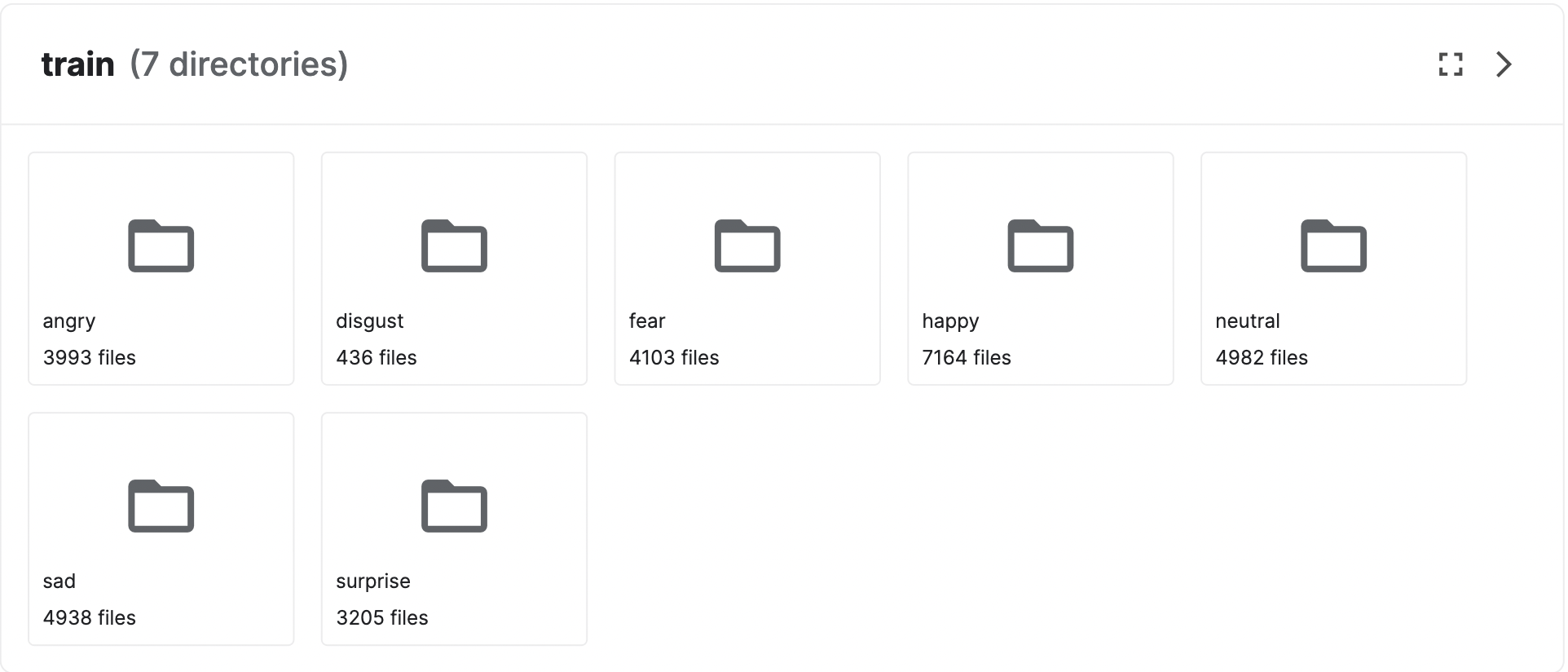
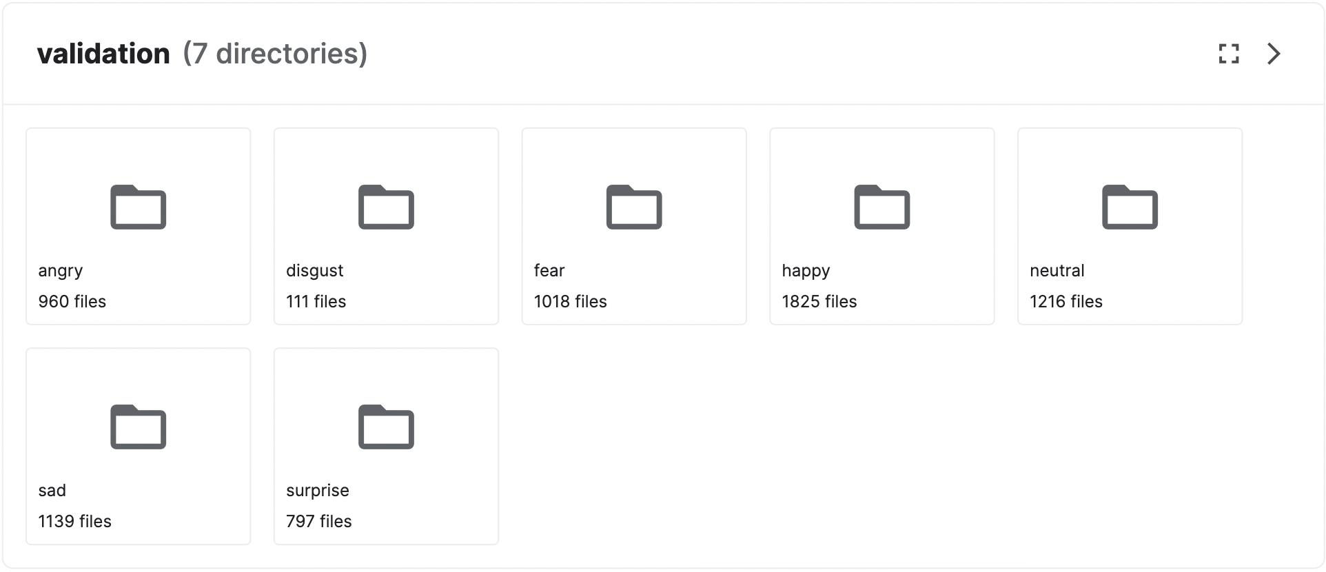
We found the dataset from the Kaggle. This dataset include the facial emotion picture for 7 classes: angry, disgust, fear, happy, neutral, sad, and surprise. It has 35.9k images in total. For the train set, the distribution for each class is the following: happy 7164, sad 4938, fear 4103, surprise 3205, neutral 4982, angry 3993, disgust 436. And for the validation set, the distribution for each class is the foloowing: happy 1825, sad 1139, fear 1018, surprise 797, neutral 1216, angry 960, disgust 111
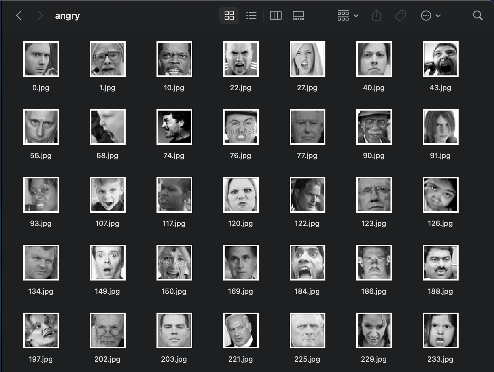
The data type of each image is (48, 48, 1) grayscale with each pixel value ranging from 0 to 255. Thus, we normalized the data by dividing every pixel by 255. The dataset is split into training, validation and testing with 7 labels
2.2 Preprocessing
2.2.1 Principal component analysis
PCA is a great technique for analyzing large dataset with a large number of features by reducing dimension. As a popular unsupervised machine learning method, the principal component direction can capture the greatest variances of the data. As we noticed that some features are redundant in our (48, 48) image, such as hair, ear, or background, performing PCA can improve algorithm efficiency and minimize information loss at the same time.
2.2.2 Results of Principal component analysis
PCA is applied to the dataset in the preprocessing stage. Since there are some unecessary features in images, using PCA can help to reduce the dimensions and hence speed up the training. The figure below shows the amount of cumulative variance covered by the numbers of components/features.
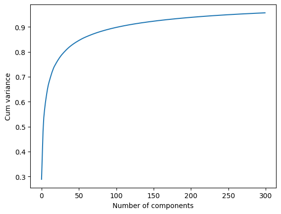
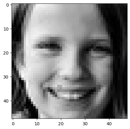
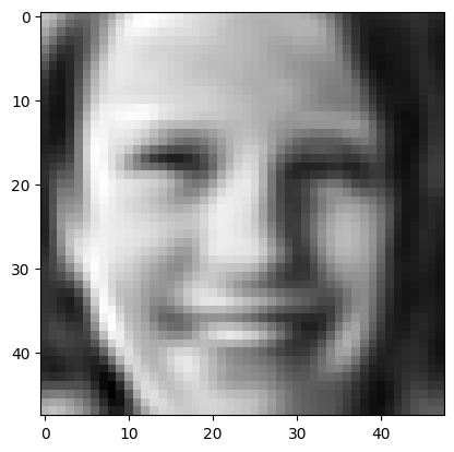
From this plot, we can spot that the “elbow” occurs at 200 features, which covers more than 90% of the variance. So, we reduce the features to 200 and then used the preprocessed images to train the models. Here is an example of an original image and after applied to PCA.
3. Methods
3.1 Neural Networks
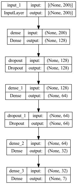
We plan to use simple Neural Network with Dense Layers on the image features after the PCA preprocessing. Therefore, we could compare the performane on the Neural Network and the Convolutional Neura Network at the end. Our Neural Network model summary looks like below.
3.2 Convolutional Neural Networks
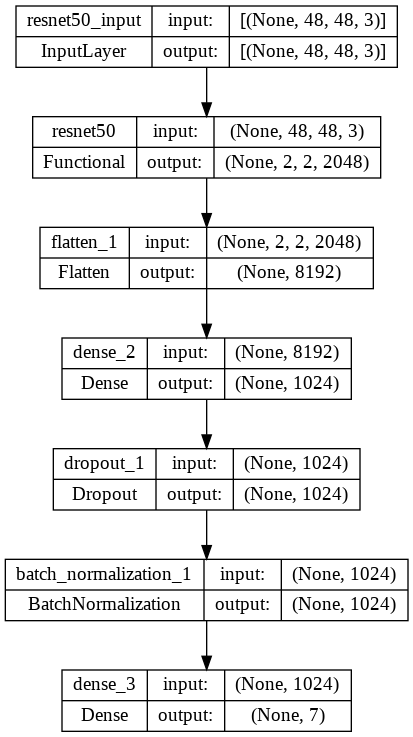
Convolutional Neural Networks(CNN) models have relative high accuracy and efficiency in image classifications. In this project, we did the transfer learning from the pre-train model. Specifically, we have ResNet, MobileNet, and AlexNet with the initial weight form the ImageNet. We also added a flatten layer, a dense layer with 1024 output and ReLu activation, Dropout Layer, BatchNormalization Layer, and finally another Dense Layer to downscale the output to 7 classes to the the orginal artiture.
Besides the transfer learning from pretrained model, we also designed a SelfNet (shown below), which consist the Conv2D Layer, BatchNormalization Layer, Dropout Layer, MaxPooling2D layer, Flatten Layer, and Dense Layer.
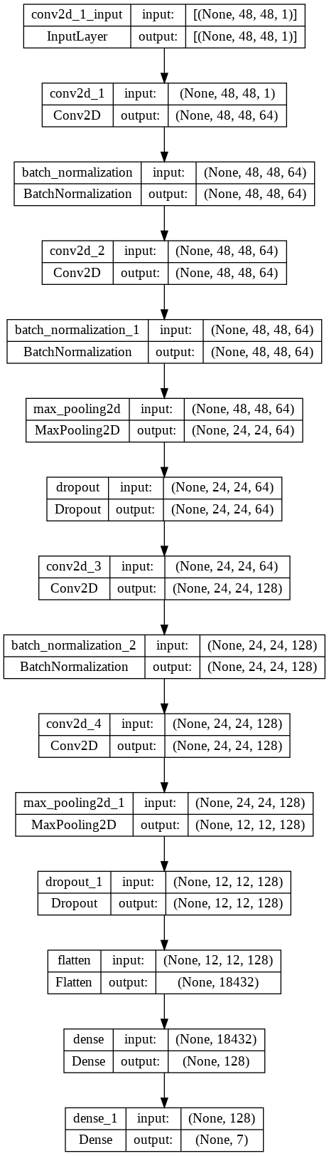
For the CNN model, we utilize slightly different preprocessing technique. To be more specific, since the pretrained model only accpet the input image with RGB three channels, However, our image dataset only have one grayscale image. Therefore, we copy the value of teh grayscale channel three times to the RGB chennel when we do the transfer learning. However, for the SelfNet, the model designed by us, we make the SelfNet be able to take the one channel image. Therefore, we did not augment the image to three channels for the SelfNet.
When we compile the CNN model, we used the RMSprop optimier with initial learning rate 0.001. Since the project is multi-classes classification problem, we choose the categorical_crossentropy as the loss funtion since.
3.3 K-nearest Neighbors
KNN is a supervised method that classifies new data based on feature similarity with the training set. We used the K Neighbor Classifier under KNN with the uniform weight to predict the classification of facial expression images in the dataset. We suspect that this may have a lower accuracy because facial cues for expressions such as anger, sadness and fear are similar.
3.4 Naive Bayes
Naive Bayes is a supervised learning method which assumes that each feature is independent, and we may focus on facial features in our NB implementation. We implemented Gaussian Naive Bayes and Multinomial Naive Bayes, but eventually chooses to implement Gaussian Naive Baiyes for higher validation accuracy. However, we suspect that accuracy may be lower because facial features are adjacent to each other, thus they may be somewhat correlated.
3.5 Support Vector Machine
SVM is a supervised learning method used for classification, regression and outliers-detection. It has the benefits of high dimensionality, memory efficiency, and versatility. For a dataset with N features, we are going to use C-Support Vector Classification with the default regularization parameter to find a hyperplane in a N-Dimensional space that classifies the dataset.
3.6 Random Forest
Random Forest is an ensemble learning method for classification. The output for the classification is the class selected by most trees. With more trees we could effectively aviod the overfitting problem. In order to address overfitting and accuracy problems of Decision Trees, we selected the Random Forest method. In addition, we limit the maximum depth of the decision trees to be 16, so instead of letting nodes expand until all leaves are pure, now it will stop at the depth of 16 to avoid overfitting. Also, we adopted the Cross-Validation method to find the optimal number of estimators.
4. Results
4.1 Neural Networks
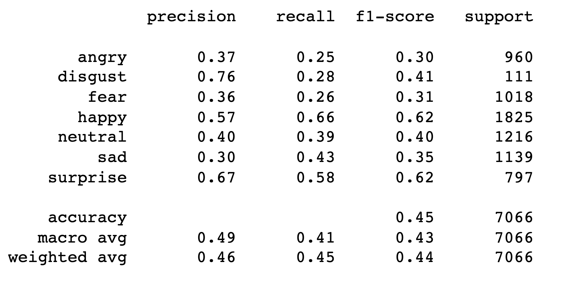
The neural network model consists 3 dense layers by Rectified Linear Unit (ReLU) layer and 2 dropout layers. We first tried to add more hidden layers to the model, but it didn’t increase the accuracy, instead, the model stated to overfitting with an increased training time. So the choice of 3 layers is better for the NN model. Then, we introduced the dropout layers with the ratio of 0.2 to help to reduce the overfitting.
Finally we have the accuracy score for the NN model is 0.4499009340503821
The confusion matrix and classification results are shown below
4.2 KNN
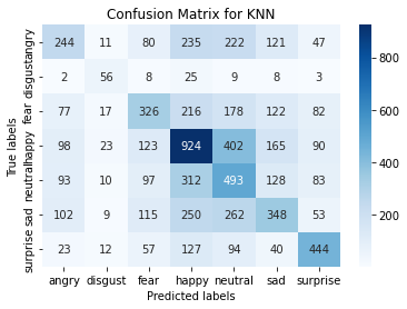
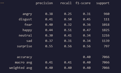
The accuracy score for the most accurate KNN model is 0.40121709595244837 which is a ball_tree algorithm using euclidean metrics with distance as the weights. The classification reports and confusion matrices are below.
The confusion matrix and the classification results of our KNN are below:
4.3 Naive Bayes
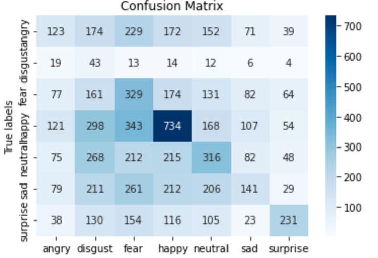
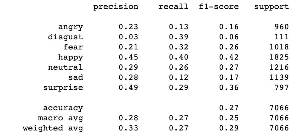
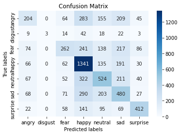
The accuracy score for the Naive Bayes model is 0.271299179167846. This model struggles with a dataset as complex as the facial recognition dataset as there are many features that can siginify more than 1 emotion. Aditionally, Naive Bayes assumes that all features are indepedent which is not the case. This model performed best with the emotons of ‘happy’ and ‘surprised’ and performed very poorly for the emotion of ‘disgust’. The issues with identifying disgust may stem from the fact that disgust was heaviily underrepresented in both the training and validation data sets. The confusion matrix and the classification of results for Naive Bayes are below:
4.4 Support Vector Machine
The accuracy score for the Support Vector Machine is 0.45655250495329747. To improve the accuracy of the model, SVM with different parameters are used to run the model. The model is runned with the kernel set to ‘linear’, ‘poly’, ‘rbf’, and ‘sigmoid’. The highest accuracy is with ‘rbf’, which is the default parameter, then followed by the ‘poly’ with accuracy of 0.3986696858194169, then is ‘linear’ with accuracy of 0.3879139541466176, and last one is ‘sigmoid’ with accuracy of 0.22459666006227003. We also tried to LinearSVC model, since it implements “one-vs-the-rest” multi-class strategy, but the accuracy is still lower than the previous one, which is 0.3819699971695443. The confusion matrix and classification report of results for SVM are below:

4.5 Random Forest
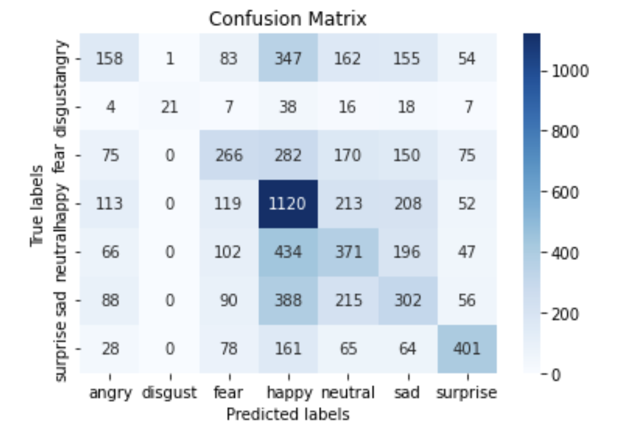
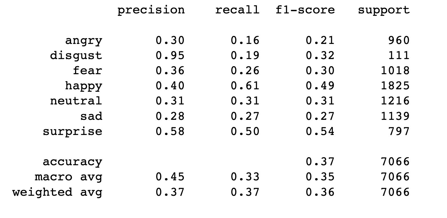
Unfortunatly the result for the Random Forest is not ideal. We only get the 0.37 accuracy with the confusion matrix and the classification report shown below
CNN
4.6 AlexNet
4.7 ResNet50
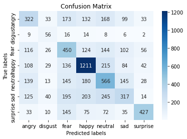
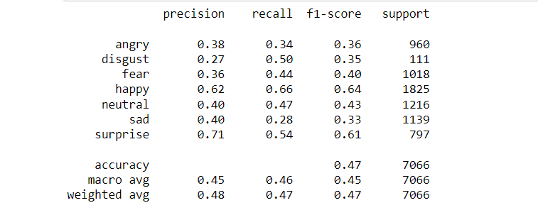
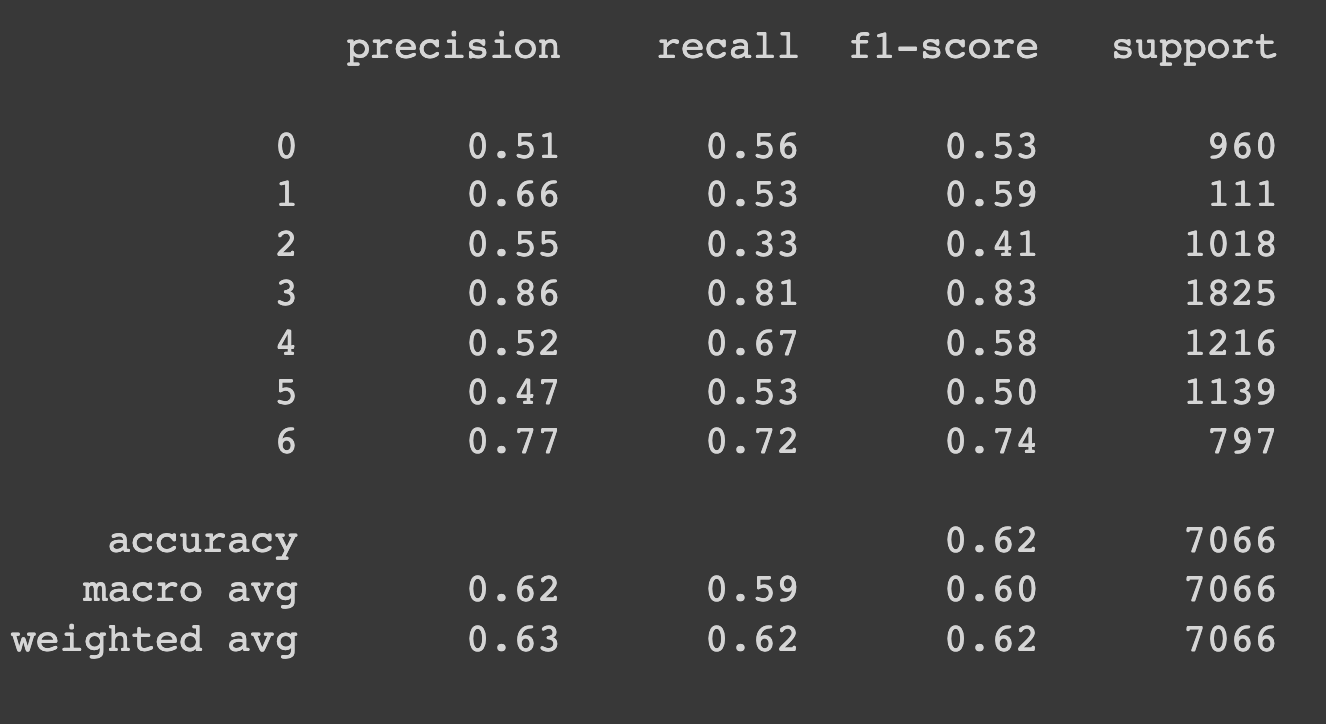
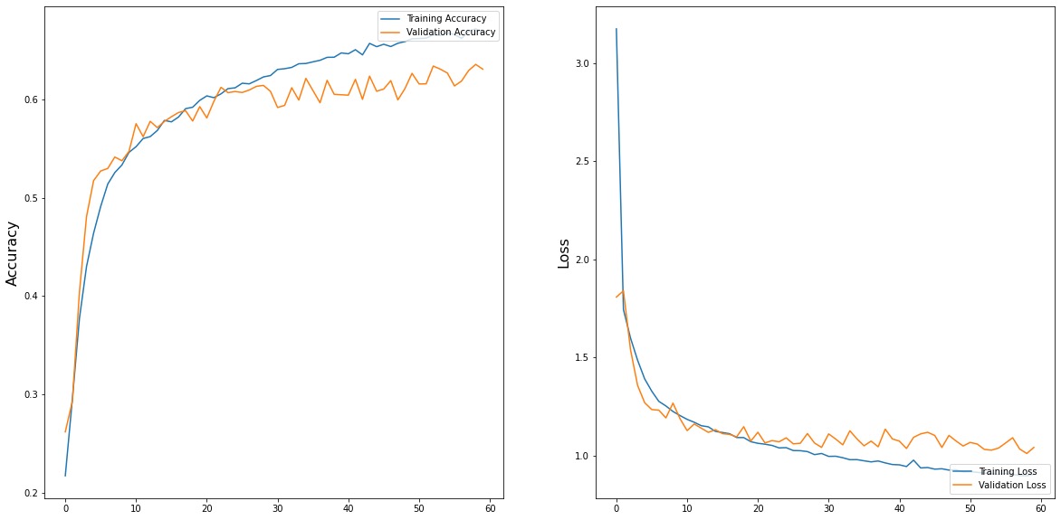
For the ResNet, we do the transfer learning for 60 epochs with the initial weight from the imageNet. The accuracy score starts to converged around 0.6 from epoch 30. Finally, we have the highest validation accuracy be 0.6219926408151712 with the history shown below. 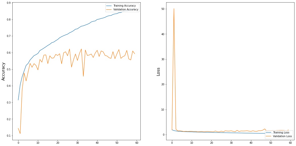
And the confusion matrix and the classification results shown below
4.8 MobileNet

4.9 SelfNet (Self Designed)
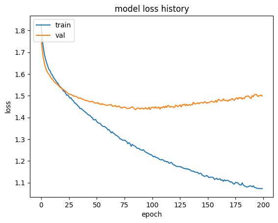
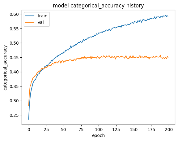
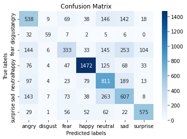
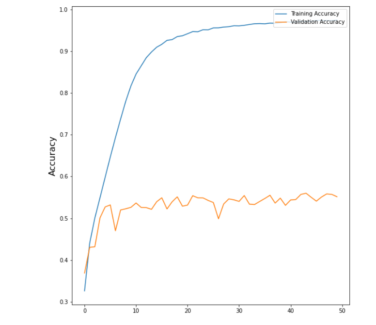
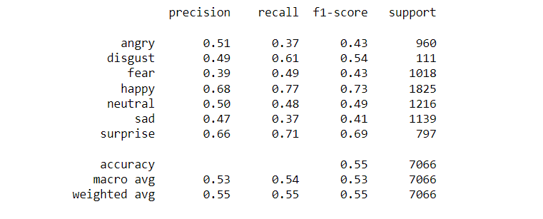
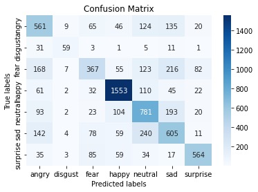
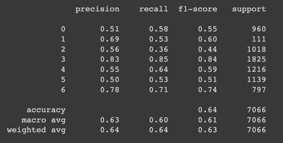
For the self-designed SelfNet we fitting the data with the random initialized weight for 60 epochs. We have the highest validation accruacy at 0.64. The fitting history is shown below.
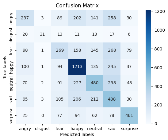
The confusion matrix and the classfication report is shown below.
5. Discussion
In this project, we studied Neural Networks, K-nearest Neighbors, Naive Bayes, Support Vector Machine, Random Forest, and CNN (ResNet, AlexNet, MobileNet, and SelfNet). We used PCA as our preprocessing method. The summary of test accuracy of all the models is presented below by a table and a chart. 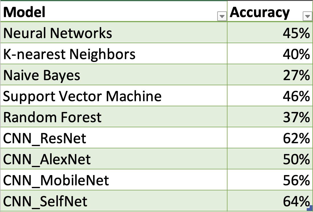
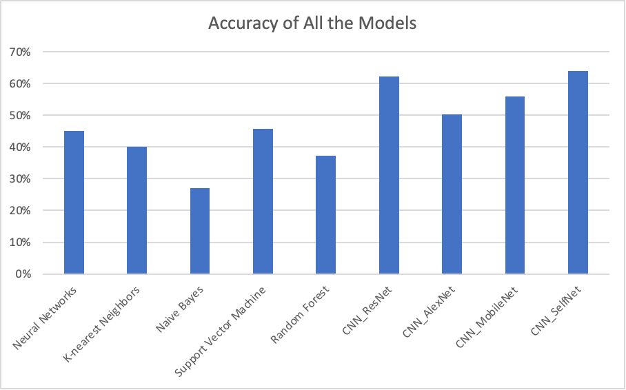
It’s clear to see that the CNN with SelfNet came out with the highest accuracy, with 64%. The other CNN models by transfer learning also performed well. This indicates Convolutional neural network is favored by the our dataset. The Naive Bayes had the lowest accuracy of 27%. There were some limitations inur dataset that hampered the ability of the different models to prduce high accuracies. One issue is that the resolution is low. Another issue is that there are watermarks for some images (Shown below).
Finally, “happy” is overrepresented in our dataset while “disgust” is underreprsented. All other emotions have approximately the same number of data points.
The CNN methods performed the best beacause they use many layers where each one learns to recognize one feature of an image. In CNN, the layers are connected as opposed to Naive Bayes where each feature is treated as independent. This distinction allows CNN to significantly outperform Naive Bayes for image classification as the different features are not truly independent. CNN also improves after each layer while Naive Bayesonly predicts which class an image belongs to based on each indepedent feature. The remaining methods all finished off with similar accuracies ranging from 40 to 50%.
6. Conclusion
Overall, we learned a lot about different machine learning methods through this project. If we were to continue wrking on this project, we would perform these next steps: 1) we would find more and better images to train the model to increase the accuracy, since some of the images are not clear and some of the emotions are not very obvious. 2) we would try to add more layers to our CNN model and fine tune the parameters. 3) we would use more visualized techniques to show how we trained the dataset.
References
Vyas, A. S., Prajapati, H. B., & Dabhi, V. K. (2019, March). Survey on face expression recognition using CNN. In 2019 5th international conference on advanced computing & communication systems (ICACCS) (pp. 102-106). IEEE.
Abdulrahman, M., & Eleyan, A. (2015, May). Facial expression recognition using support vector machines. In 2015 23nd signal processing and communications applications conference (SIU) (pp. 276-279). IEEE.
Sebe, N., Lew, M. S., Cohen, I., Garg, A., & Huang, T. S. (2002, August). Emotion recognition using a cauchy naive bayes classifier. In Object recognition supported by user interaction for service robots (Vol. 1, pp. 17-20). IEEE.
Timeline

Contribution table
| Member | Contribution |
|---|---|
| Parth | Timeline, Github Page, Proofreading, Naive Bayes, Discussion, Final Presentation |
| John | Discussion, Github Page, Proofreading, KNN |
| Bruce | Method, Video, Potential Results, MobileNet, AlexNet, Final Presentation |
| Zhaodong | Dataset, Slides, Discussion, Github Page, PCA, Random Forest, SelfNet, ResNet, Final Presentation |
| Yanzhu | Introduction, Problem Statement, Methods, PCA, SVM, Discussion, Final Presentation |
Video
Please Check our midterm video via this link
Please Check our final video via this link