Convolution and Hybrid Images
Table of Contents
Convolution and Hybrid Images
Overview
To write an image filtering function and use it to create hybrid image based on paper. Hybrid images are static images that change in interpretation as a function of the viewing distance. To create a hybrid image, I need to blend the high frequency portion of one image with the low-frequency portion of another
Implement Convolution with NumPy
Gaussian Kernels
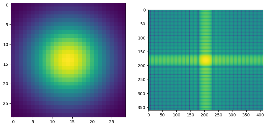
Gaussian filters are generally used to blur the images. In this step, I implemented the Gaussian kernels as shown below.
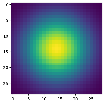
After applying this Gaussain filter to an image, it blurs this image 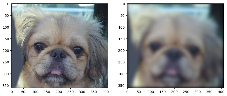
Convolution
Convolution (or filtering) is a fundamental image processing tool. In this section, I implemented my_conv2d_numpy() based on the equation
where f=filter (size k x l)I = image (size m x n), In my_conv2d_numpy(), I firstly do a padding for the input image according to the the filter.shape[0]//2 and filter.shape[1]//2 to ensure the size of the image would not change after filtering. Then, I use nested for loop to do the element-wise multiplication between the filter and image. Then, take the sum of the multiplication as the result for the value in that index
Below, there are some exmaple of differents kernels
 |  |
| Identity Filter | Box Filter |
 |  |
| Sobel Filter | Discrete Laplacian filter Filter |
Hybrid Images
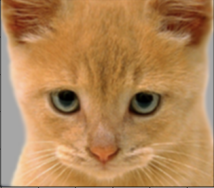
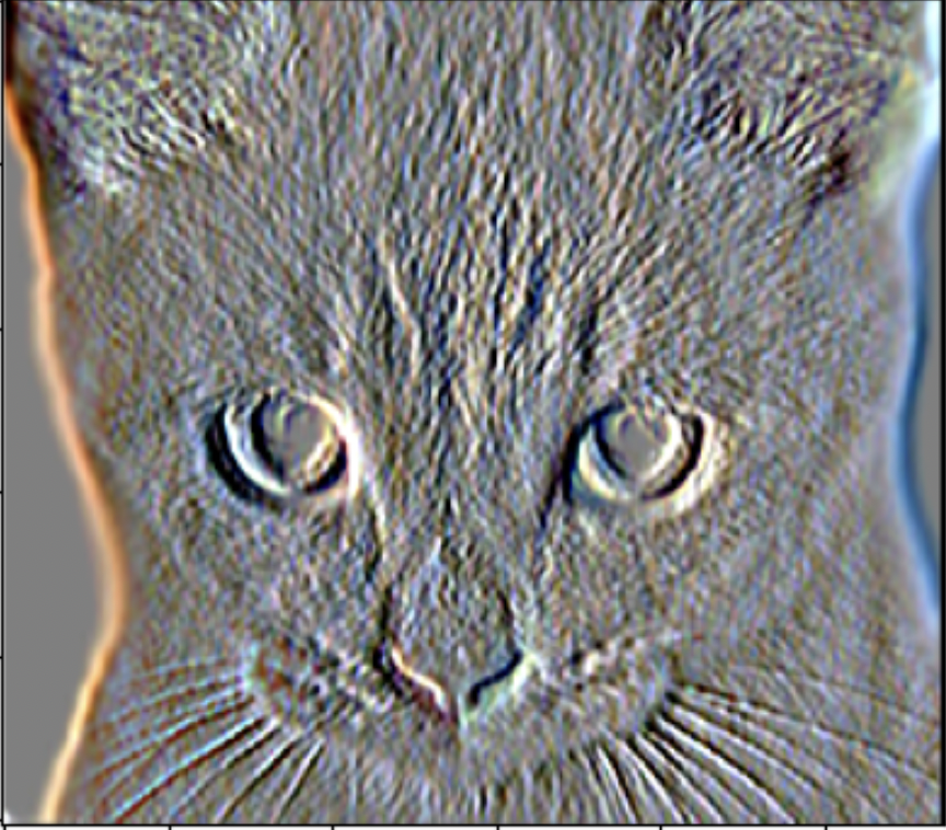
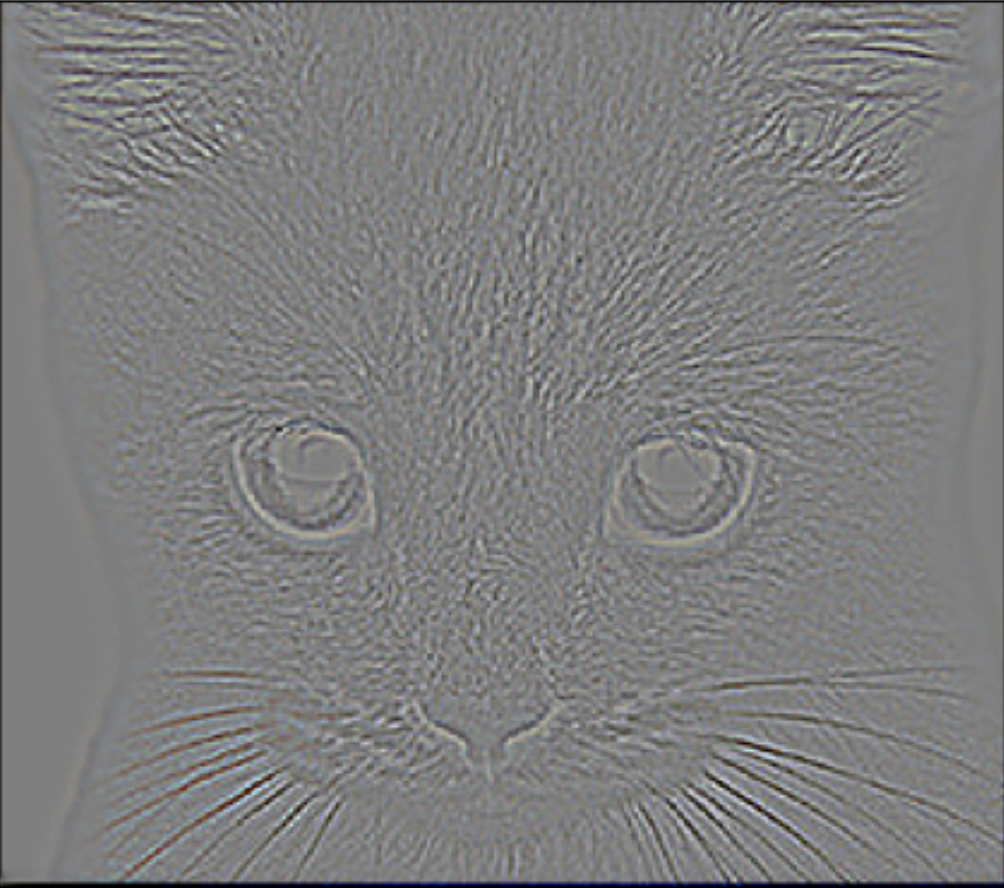
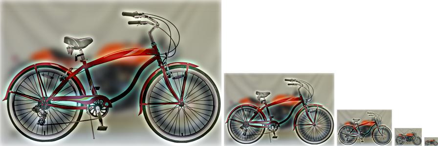
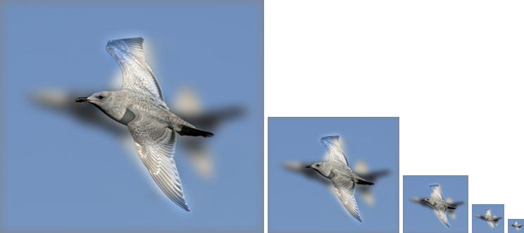
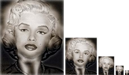
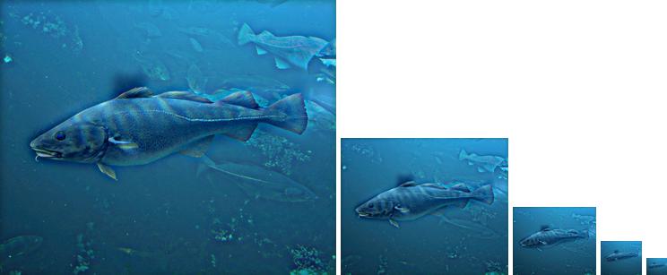
Hybrid image (images give you different view when the distance changes) is the sum of a low-pass filtered version of one image and a high-pass filtered version of another image. To get the hybrid image, I do the following three steps
- Step 1: Get the low frequencies of image1 Using
my_conv2d_numpy(image1, filter) - Step 2: Get the high frequencies of image2 by subtracting the low frequencies from the original images
- Step 3: Get the hybrid image by add the low frequencies of image 1 and the high frequencies of image 2 (Note: we need to clip the final image to make sure that the value is in the proper range [0,1], using the
numpy.clip())
Below are some examples: 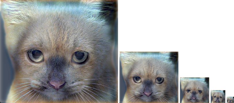
Frequency Domain
Frequency Domain Convolutions
The Fourier transform of the convolution of two functions is the product of their Fourier transforms, and convolution in spatial domain is equivalent to multiplication in frequency domain. Therefore, we could do the convolution in the spatial domain.
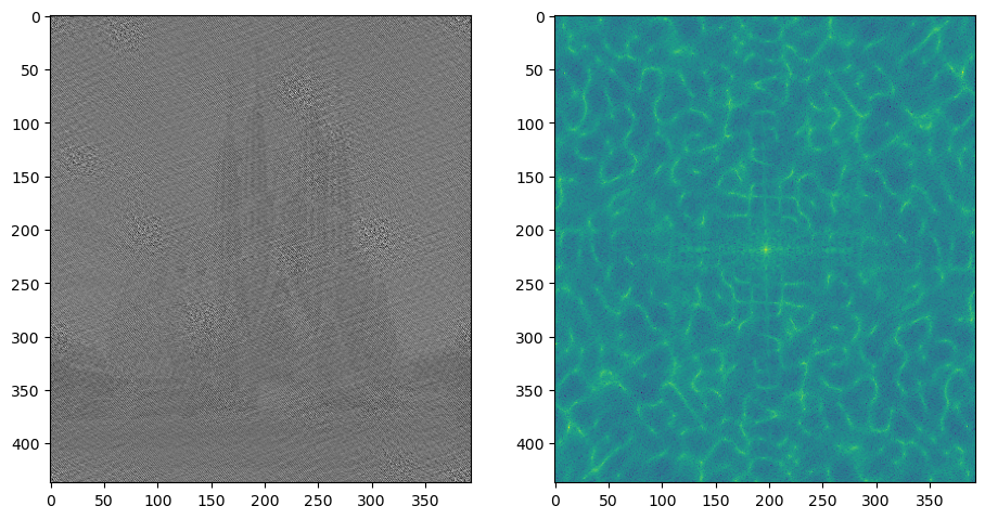
I have the orgial image and kernal shown below in Spatial and Frequence Domain seperately. 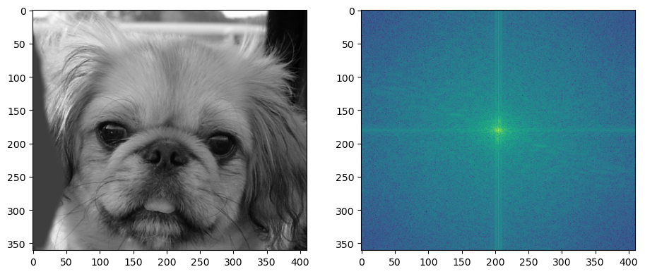
After the multiplication, I get the following result 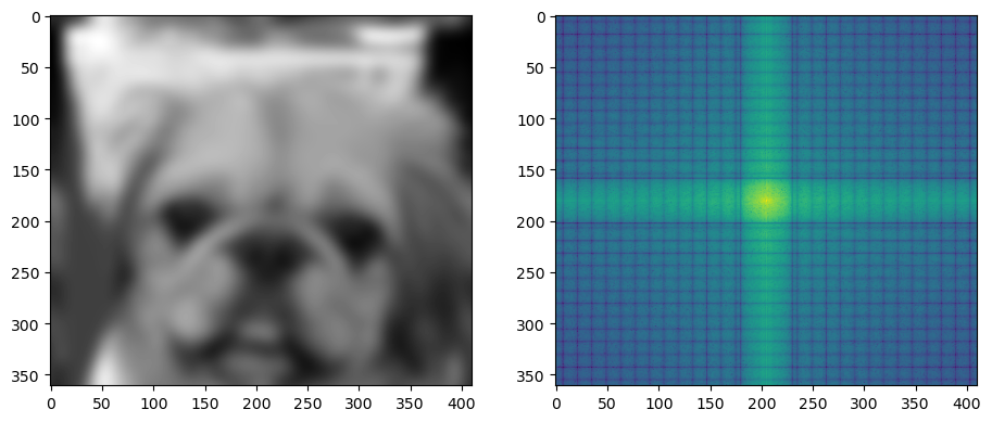
Frequency Domain Deconvolutions
The Convolution Theorem refers the convolution in spatial domain is equivalent to the multiplication in frequency domain. With that idea, when comes to the invert the convolution, we could think about the division in the frequency domain. This idea leads to the deconvolution.
For the above example, after the frequency domain division, we get the following the result 
Limitation of Deconvolutions
There are two factors that the deconvalutions mostly does not work in real world
- First factor is that in the real world, we mostly do not know the filter
- The second factor is that for some filter (like zero filter), it is almost impossible to do deconvolution
Also, the deconvutions are very sensitive to noise.
Here is a example, provided the following image with its kernel 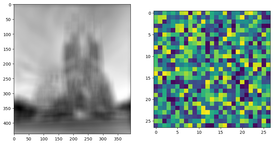

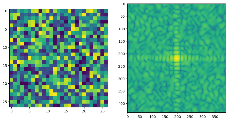
We could get the good deconvultion by doing the frequency domain division, shown below 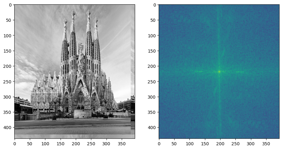
However, if we add the salt and pepper noise, we could only get this